Analysis of causal dependencies

Operational risks pose challenges for all companies. In particular, their high complexity and numerous causal dependencies make the management of these risks difficult.

While companies are already using methods for recording and measuring operational risks, these methods are still only available in rudimentary form for the evaluation of measures, the analysis of causal causes or the consideration of alternatives.
In fact, however, the analysis of causal dependencies is essential in order to be able to make decisions at all! Only if the consequences of a measure can be estimated, appropriate decisions can be made and alternatives can be evaluated. Only then are methods such as "prescriptive analytics" useful at all.

In recent decades, there has been accordingly considerable progress in the field of Causal Inference. It is now possible to quantify the actual influence of interventions on the basis of available data. Furthermore, it is possible to retrospectively (counterfactually) determine causes and evaluate alternatives.

In the following, the methods of causal inference and their possible applications in OpRisk management are explained on the basis of various use cases. Among other things, they can be used to objectively evaluate the effectiveness of controls and check mitigation measures.

Operational Risks

The business activities of every company entail specific operational risks (OpRisks). These can be caused by

• humans (e.g. internal oder external fraud)
• processes (e.g. control deficiencies)
• systems (e.g. system crashes) or
• external events (e.g. natural catastrophes)

Legal risks also represent a further subgroup. OpRisks can often result in reputational risks, which can lead to lost sales and the loss of key personnel, among other things.

Loss events

When operational risks occur, they lead to operational losses. These can be considerable. Prominent cases include, among others

• fraud cases (e.g. Diesel affair)
• hacker attacks (e.g. Solar Winds)
• computer viruses (e.g. MyDoom)
• natural disasters (e.g. Fukushima)

In addition, however, every company is exposed to many small damages that have their effect due to their frequency, such as system crashes, terminations of key personnel, incorrect bookings, etc.

Classification

The Basel II banking regulations divide OpRisks into the following seven categories, which are also relevant for other industries:

1. internal fraud: misappropriation of assets, tax evasion, intentional mislabeling of positions, bribery
2. external fraud: theft of information, hacking, third-party theft and forgery
3. employment practices and workplace safety: discrimination, workers' compensation, employee health and safety
4. customers, products and business practices: market manipulation, antitrust, unauthorized trading, product defects, breaches of fiduciary duty, account changes
5. propertydamage: natural disasters, terrorism, vandalism
6. business interruptions and system failures: supply interruptions, software failures, hardware failures
7. execution, delivery and process management: data entry errors, accounting errors, missed mandatory reports, negligent loss of client assets

Current analysis of operational risks

Data acquisition

The basis for quantification is the systematic recording of internal loss events that have already occurred as well as near misses. These provide a historical basis for estimating future losses.

In addition to the internal data, anonymized external data are also available. These increase the database, but generally contain less information than the internal databases. In addition, internal audits often have detailed information on past losses.

Risk quantification

A common classification of OpRisks is based on their frequency and extent. A summary can then be presented, for example, by means of a heat map.

Risk indicators such as value at risk (VaR) can be used to quantify risks. Scenario analyses are also possible, for example in the context of stress tests. (Monte Carlo) simulations are also used here.

A difficulty here lies in the determination of the parameters, which are often provided with a bias (e.g. selection). There is also the danger of confusing correlation with causality.

Current causal analyses

Bowtie diagrams are a common method for modeling causal relationships in the OpRisk area. Here, the causes (and the corresponding controls) of a possible loss as well as the consequential losses are depicted in the form of a diagram, which generally has the shape outlined on the right. These diagrams can provide a qualitative starting point for causal relationships.

Fig. 01: Bowtie diagram (schematic)

Even beyond this, causal relationships are generally only examined qualitatively. Quantitative analyses are limited to risks and correlations as well as scenario considerations based on observations and assessments.

Thus, neither causes can be determined objectively, nor measures (interventions) can be evaluated, nor alternative courses of action can be investigated quantitatively. This requires extra-statistical methods such as those provided by causal inference.

Causal Inference

Background

The methods of causal inference have been increasingly used for some years, especially in the biomedical field, where there is sometimes talk of a "causal revolution".

This makes it possible to identify actual causes and to separate correlations from causalities.

This allows the effect of possible measures to be estimated from the observations without having to implement the measures. In addition, it is possible to determine (necessary and/or sufficient) causes retrospectively.

Do-Calculus and Counterfactuuals

With the do-calculus, it is possible to estimate the effect of interventions on the basis of observations, without having to carry out the - often not even possible or ethically justifiable - interventions themselves. For some simple causal relationships, formulas can be derived to calculate ratios. Do-operations differ from statistical conditioning (i.e., filtering) because the changes here are applied (notionally) to all observations.

Counterfactuals are another subfield. Here we investigate how a result y(x) would have turned out with real y₁(x₁), if x were instead (fictitiously) unequal to x₁.

Key figures

Causal inference methods are extra-statistical because they require knowledge about causal relationships that is external to the data and can be represented, for example, by means of graphs (more precisely: directed acyclic graphs) (see below).  The determination of causal relationships requires subject matter expertise and can at best be verified with the help of observed data, but not inferred from them.

Once this has been done, the following relevant key figures, among others, can be calculated - depending on the causal case (see also Info Box 01: Glossary):

• Conditional Probability (PE): the conditional (observed) probability P(Y | X) of the result Y under the condition X. The conditional probability corresponds to a filtering of the data sets.
• Total Effect (TE): the change in probability for Y after implementation of an intervention  X₀ → X₁: P(Y | do(X) = X₁) – P(Y | do(X) = X₀). The determination of the total effect requires causal considerations, since for this the intervention must be carried out (mentally) for all individuals and the effect derived from this.
• Effect of Treatment on the Treated (ETT): here, the extent to which a certain cause has actually contributed to a certain effect is considered. For this purpose, the individuals are considered for whom a cause X = 1 led to an effect Y = 1. Subsequently, it is determined – counterfactually – to what extent the observed effect would also have occurred for these individuals with a different cause X = 0. The ETT is the difference between the two. 
• Probability of Necessity (PN): Probability that Y would not have occurred in the absence of X, but when X and Y actually occurred. This parameter is often relevant for legal questions.
• Probability of Necessity and Sufficiency (PNS): Measure of sufficiency as well as necessity of X for the generation of Y
• Excess Risk Ratio (ERR): similar to PN, but minus the confounding bias: (P(Y|X) – P(Y|X')) / P(Y|X)

The following ratios are relevant for the mediation case, i.e., for the case where a variable X affects Y both directly and indirectly via a variable Z ("mediator"):  X → Y  and  X → Z → Y

• Controlled Direct Effect (CDE): Change of result Y when direct parameter X is changed and mediator Z is fixed at the same time.
• Natural Direct Effect (NDE): Change of the result Y with change of the direct parameter X and free development of the mediator Z. In contrast to the Total Effect, the connection from X to Z is mentally "cut", i.e. Z develops completely "naturally". The calculation of the NDE requires counterfactual considerations. The NDE indicates the extent to which the effect is solely due to the direct cause when the mediator is removed, i.e., the extent to which the mediator can be dispensed with.
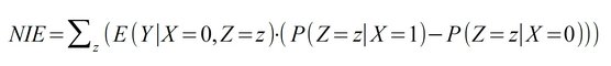
• Natural Indirect Effect (NIE): Change of the result Y with change of the mediator Z and free development of the direct parameter X. The connection from X to Z is here mentally "cut", i.e. X evolves completely "naturally" and Z is fixed independently. The calculation of the NIE requires counterfactual considerations. The NIE indicates the extent to which the effect occurs solely through the indirect agents when the direct cause is eliminated, i.e., the extent to which the direct cause can be dispensed with.

Analysis of non-trivial relationships

Confounding / Backdoor

In this case, a variable X influences a variable Y. Both X and Y are additionally influenced by a variable Z ("confounder").

Fig. 02: Confounding / Backdoor

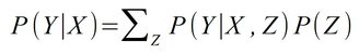
To calculate the effect of interventions on X (i.e. P(Y | do(X))) – and thus of TE – the so-called backdoor formula is used. 
This exploits the fact that Z is a causal "backdoor" from X to Y. Accordingly, Z is summed up: 

Frontdoor

Here, both the variable to be changed X and the result variable Y are influenced by a variable U. However, U is unknown.
In addition, there exists a variable Z that is not influenced by U and "intercepts" the influence of X on Y.

Fig. 03: Frontdoor

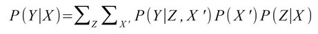
In this case, the influence of X on Y – i.e. P(Y | do(X))) and thus the Total Effect TE – can be determined by frontdoor formula even if U is unknown:

 
Mediation

In this case, the effect of X on Y is both direct and indirect via a mediator Z.

Fig. 04: Mediation

While the calculation of the TE is trivial, the determination of the direct and indirect effect requires more complex formulas, some of which are based on counterfactual considerations.

For the mediation case, this allows several other ratios to be calculated, such as ERR, ETT, PN, PNS, CDE, NDE, and NIE (for index nomenclature of counterfactuals, see Glossary):

ERR = (P(Y | X) – P(Y | X')) / P(Y | X)
ETT = E(Y₁ – Y₀ | X = 1)
PN = P(Y₀=0 | X=1, Y=1)
PNS = P(Y₁=1, Y₀=0)
CDE = E(Y | X=1, Z=0) – E(Y | X=0, Z=0)
     

Instrumental variables

In the case of linear dependencies, the analysis possibilities expand considerably.

This is also the case for instrumental variables. Here, the joint influence U is unknown, but X is also influenced by a known variable Z.

Fig. 05: Instrumental variables

In the case where Y depends linearly on Z with a regression parameter r_ZY and X in turn depends linearly on Z with a regression parameter r_ZX, the dependence of Y on X is:
r_XY = r_ZY / r_ZX

Applications in OpRisk Management

Fictitious example

Situation: fires break out in a company all the time. That's why some departments conduct elaborate fire safety training courses, which include practicing the effective use of fire extinguishers. In fact, in relative terms, fires decrease from 56% to 45% compared to departments without training. The calculated total effect is 11%. However, it can also be seen that fire extinguishers were used more often (64%) in the trained departments (again, in relative terms) than in the non-trained ones (22%).

Fig. 06: Example fire extinguishers

Tab. 01: Use of fire extinguishers

Question: management is therefore considering cancelling the costly training sessions and only practicing the operation of the fire extinguishers. How would the effect of this be assessed?

Solution: this is a mediation case. Relevant is the counterfactual consideration of how much the fires would be reduced if the use of the fire extinguishers corresponded to the level of knowledge of the training, but the training itself had not taken place. The corresponding Natural Indirect Effect is -3%. Therefore, reduced training should be discouraged, as it would even be (slightly) counterproductive. The use of fire extinguishers is only effective in combination with the training provided.

OpRisk Usecases

Data theft by hackers

Fig. 07: Data theft by hackers

• Basel II number: 2
• Causal model: hacker steals data either directly or later via an installed trapdoor. The latter can also be done via the installation of malware.
• Possible question(s): where are the main weak points? With scarce resources, should investment be more in malware or hacker mitigation?
• Identifying the TE hacker is trivial. Otherwise, mediation cases are available and can be calculated as follows:
  • NDE malware: conditioning on hacker and trapdoor.
  • NIE malware: mediation formula with confounding and conditioning hacker.

Internal Fraud

Fig. 08: Internal Fraud

• Basel II number: 1
• Possible question(s): are deficiencies in the recruiting process the cause of fraud and to what extent does the working atmosphere also contribute to it? What should be done about it?
• Causal model: (unknown) recruiting deficiencies lead to fraud-prone individuals being hired. These individuals either try to cheat directly or only after incidents that result in warnings, for example. The latter are also favored by the working atmosphere. If control deficiencies are also present, the fraud is "successful".
• For the analysis of personal causes, control deficiencies can be left aside, since there is no causal path. If linear relationships are also assumed, both the share of the working climate in fraud cases and recruiting deficiencies can be measured.

Project Risks

Fig. 09: Project Risks

• Causal model: deficiencies in project management lead to too tight a schedule. As a result, the work per employee increases too much and the project fails because deadlines cannot be met. In addition, project management deficiencies also lead directly to the failure of the project, for example due to misallocation.
• Possible question(s): should project management in general be improved? To what extent are external circumstances to blame for failed projects?
• Since project management deficiencies usually cannot be measured directly, the frontdoor criterion can be used here. With this it is possible to determine the corresponding TE through the tight time planning.
• Key risk indicators include time recording and customer feedback.

Incorrect bookings on holidays

Fig. 10: Incorrect bookings on holidays

• Basel II number: 7
• Causal model: employees are absent on public holidays and therefore also experienced employees. In addition, there may be more bookings or more complex bookings. Both can result in time or complexity issues, ultimately leading to incorrect bookings.
• Possible issue(s): should the process for approving vacation days be reconsidered? Are more or more experienced employees needed on holidays?
• The calculation of the TE of 1, 2 and 3 is trivial. For the TE of 4, the backdoor criterion must be applied. For 2 there is also a mediation case and NDE and NIE can be determined accordingly.

Consequences Data Loss

Fig. 11: Consequences Data Loss

• Causal model: Here, the consequences of a loss that has occurred are considered. A loss of data can lead to a loss of intellectual property as well as to legal consequences (lawsuits) and reputational damage. The former can lead to compensation payments and the latter to a drop in sales.
• Should litigation with regard to reputational damage be avoided despite good prospects of success?
• To determine the TE of legal consequences, the backdoor criterion should be applied. Furthermore, there is a mediation case with the legal consequences as mediator; accordingly, NDE and NIE can be determined.
• This case is particularly relevant for insurance companies, as they are likely to have corresponding data.

Non-ergonomic armchairs

Fig. 12: Non-ergonomic armchairs

• Basel II number: 3
• Causal model: presumably due to policy deficiencies, unsuitable office chairs are purchased, which lead to back problems and which in turn lead to lawsuits. At the same time, the general poor economic situation of the company could also be responsible for the cheap chairs and the lawsuits.
• Possible question(s): should the occupational safety policy be revised?
• Provided the root cause is unknown, the front door criterion lends itself to identifying the TE of the problematic armchairs.
• This case is particularly relevant for insurance companies as they are likely to have relevant data.

External Fraud

Fig. 13: External Fraud

• Basel II number: 2
• Causal model: here, external fraudsters manipulate internal MA via social engineering, who then commit errors through negligence, resulting in damage. In addition, damage can also be caused directly via other channels.
• Possible question(s): should employees be trained first or should a risk assessment be conducted?
• If the actual cause is unknown, the front door criterion can be used to identify the TE caused by the social engineering of the employees and to possibly close this security gap through training.

Aggressive Sales

Fig. 14: Aggressive Sales

• Basel II number: 4
• Causal model: Presumably due to compliance deficiencies, managers are tempted to set too hard sales targets, which increase the pressure on employees, who then sell too aggressively. At the same time, compliance deficiencies can also lead directly to aggressive selling.
• Possible question(s): Should compliance rules be revised? Should individual managers be held responsible?
• If the root cause is unknown, the frontdoor criterion can be used to identify the TE of the targets that are too heavy. Unaccountable portions are likely to be due to compliance deficiencies.

Valuation Model Error

Fig. 15: Valuation Model Error

• Basel II number: 4
• Causal model: compliance deficiencies lead to neither proper training of employees nor clean validation processes; both – together with a direct effect – lead to model errors.
• Possible question(s): should compliance be strengthened? Do new specialists need to be hired or employees need to be trained more? 
• If the TE of the know-how deficiency is to be determined, the backdoor criterion is to be applied to both the compliance and validation deficiencies. If the TE of the validation deficiency is to be determined, the backdoor criterion is to be applied analogously to both the compliance and the know-how deficiencies. 

Unauthorized Data Transmission

Fig. 16: Unauthorized Data Transmission

• Causal model: There is neither anonymization nor sufficient controls to prevent disclosure.
• Possible issue(s): Is employee training required? Does the anonymization concept need to be revised?
• Determining the TE in the case described is trivial. 
• The only thing to be careful about is not conditioning on unauthorized transfer, since this is a collider (→ ←) and conditioning on this would lead to a spurious correlation between blocking and anonymization deficiencies.

System Crash

Fig. 17: System Crash

• Basel II number: 6
• Causal model: both software innovations and support and service provider issues, as well as hackers/malware, can lead to system crashes via the paths outlined on the right.
• Possible question(s): what needs to be addressed next: Antimalware protection, contracting with new service providers, revising interfaces, replacing outdated software packages?
• Despite its high complexity, this model can also be broken down to simpler backdoor and mediation cases. These can then be analyzed using the usual criteria.
• KRIs can include installation effort (for incompatibilities), number of updates/patches (for updates), or news and ratings (for shutdown of external provider).

Erroneous Entries

Fig. 18: Erroneous Entries

• Basel II number: 6
• Causal model: incorrect entries can result from miscommunication, time pressure or lack of know-how. The first two items are more likely to occur with new employees, while holidays may encourage the latter.
• Possible issue(s): is there a need to improve employee onboarding? Do employees need training in general? Do holiday regulations need to be revised?
• Determining the TE of 1 and 2 is trivial. for 4, two backdoors (3 and/or 6 as well as 5) need to be considered. 3 and 5 represent mediation cases; accordingly, the respective NDE and NIE can be determined.

Further references

• Pearl, J., Mackenzie, D. (2018). The Book of Why: The New Science of Cause and Effect (1. Aufl.). Basic Books.
• Pearl, J., Glymour, M., Jewell, N., P. (2016). Causal Inference in Statistics: A Primer (1. Aufl.). Wiley.
• Girling, P., X. (2013). Operational Risk Management: A Complete Guide to a Successful Operational Risk Framework (1. Aufl.). Wiley.