

300 suppliers, six risk characteristics, and a single question: Which suppliers are truly similar? Cluster analysis attempts to reveal hidden structures in multidimensional data—without predetermining which groups should exist. This is particularly appealing in risk management: Instead of assigning a traffic light rating to each metric in isolation, entire risk profiles can be identified. However, for mathematical proximity to translate into a reliable management statement, the distance measure, scaling, number of clusters, and validation must be selected methodologically sound.
Why a traffic light system is often insufficient
Risk reports are often structured one-dimensionally: Poor creditworthiness—red. Weak delivery reliability—red. High single-source dependency—also red. This logic is simple, but it breaks down a multidimensional risk profile into individual warning lights. Two suppliers can have the same credit rating and yet be critically different: One supplies a standard part from within the country that can be easily replaced, while the other supplies a custom component with a nine-month lead time from a geopolitically exposed region.
Cluster analysis takes a different approach. It does not first ask whether a single data point exceeds a threshold, but rather which observations are similar across multiple characteristics. In statistics, it is classified as a method of exploratory multivariate analysis; in machine learning, it is usually categorized as unsupervised learning. Thus, there is no predefined target variable—such as "failure yes/no"—that the model is supposed to learn. The groups emerge from the structure of the data itself.
This makes the method well-suited for diagnostic analytics: it helps to understand patterns and structure in complex data. However, it does not yet provide a causal diagnosis. A cluster initially states: "These objects are similar according to the chosen mathematical definition." Why they are similar and what actions should follow from this remains a task for domain-expert interpretation. [cf. Romeike / Wieczorek 2026]
What is a cluster, mathematically speaking?
Let's represent each supplier as a point in a multidimensional feature space. With six risk features, each supplier has six coordinates. A clustering method then searches for groups in which the distances between the points are small and the distances to other groups are as large as possible. What "small" means depends on the distance metric.
For metric data, the Euclidean distance is often used. After standardizing the features, it is defined for two suppliers i and l as:
d(i,l) = √[ Σⱼ (zᵢⱼ - zₗⱼ)² ]
The formula appears straightforward, but it contains a key modeling decision: It assumes that differences across all considered variables can be meaningfully combined. This is precisely why data preparation is not a secondary step, but rather an integral part of the method.
Step 1: First, make the scales comparable
A failure probability ranging from 0 to 10 percent, a delivery time variation ranging from 0 to 30 days, and a cyber exposure score ranging from 0 to 100 exist on completely different scales. If raw values were directly used in a Euclidean distance calculation, variables with large numerical ranges could dominate the grouping—regardless of their business significance.
A standard solution is z-standardization. For each value, the mean of the variable is subtracted, and the result is then divided by its standard deviation:
zᵢⱼ = (xᵢⱼ - x̄ⱼ) / sⱼ
Accordingly, a z-score of +1 roughly means: one standard deviation above the mean. This makes the variables more comparable in mathematical terms. At the same time, an important governance issue arises: If three nearly identical financial metrics, but only one cybersecurity metric, are included in the analysis, the "finance" category effectively receives greater weight. Feature selection is therefore always a form of risk modeling as well.
Step 2: Choose a method that fits the data structure
K-means is one of the best-known clustering methods. MacQueen described the approach in 1967 as an efficient method for dividing observations into k groups [see Romeike / Wieczorek 2026, p. 151]. In simple terms, the algorithm searches for k centers and assigns each point to the nearest center. The centers are then recalculated. This process is repeated until the solution hardly changes at all. The sum of the squared distances within the clusters is optimized:
min Σc Σᵢ∈C_c || zᵢ - μ_c ||²
This makes K-means fast and easy to interpret, but not universally applicable. The method tends to favor compact, roughly spherical clusters and is sensitive to outliers. Furthermore, k must be specified in advance. For groups that vary greatly in size or are non-convex, other methods may be more suitable.
A classic alternative is hierarchical cluster analysis. In the agglomerative approach, each observation starts as its own cluster; subsequently, those groups that best match according to a chosen criterion are merged step by step. The Ward method minimizes the additional loss of homogeneity within the groups at each merger [see Ward 1963]. The result can be represented as a dendrogram—a "family tree" of similarities (see Fig. 01).
![Fig. 01: Dendrogram of hierarchical cluster analysis—step-by-step merging of similar objects using the Ward method [Source: Author's own figure based on illustrative data]](/fileadmin/_processed_/a/8/csm_Figure-01_Data-Analytics_20261002_ce8dfd9887.png "Fig. 01: Dendrogram of hierarchical cluster analysis—step-by-step merging of similar objects using the Ward method [Source: Author's own figure based on illustrative data]") Fig. 01: Dendrogram of hierarchical cluster analysis—step-by-step merging of similar objects using the Ward method [Source: Author's own figure based on illustrative data]
Fig. 01: Dendrogram of hierarchical cluster analysis—step-by-step merging of similar objects using the Ward method [Source: Author's own figure based on illustrative data]
If the data includes categories in addition to metric variables—such as region, certification status, or procurement type—a simple Euclidean distance is often no longer appropriate. In such cases, methods such as Gower distances in combination with hierarchical procedures or Partitioning Around Medoids may be considered [see Romeike / Wieczorek, p. 169]. The methodological rule of thumb is: Do not force the algorithm onto the data; instead, adapt the data type to the algorithm.
Step 3: How many clusters are "correct"?
The uncomfortable answer is: Most of the time, there isn't a single objectively "correct" number. A clustering solution is a model of the data structure. Different levels of granularity can all be meaningful at the same time—much like a map shows different details depending on the scale.
Nevertheless, there are quantitative guidelines. The elbow method examines how much the variance within the clusters decreases as k is increased. Rousseeuw's silhouette method compares, for each observation, its proximity to its own cluster with its proximity to the nearest foreign cluster. The silhouette value ranges from -1 to +1; high positive values indicate a well-separated assignment. The gap statistic developed by Tibshirani, Walther, and Hastie compares the observed cluster structure with a suitable reference distribution that lacks distinct clusters [see Tibshirani / Walther / Hastie 2001].
The key point is this: No single metric should be the sole deciding factor. A good clustering solution should be statistically plausible, robust to small changes in the data, interpretable in a domain-specific context, and usable for decision-making. Four mathematically sound clusters that no one in the company can explain or treat differently are analytically interesting—but operationally worthless.
Methodological Guide for Practice
1. Define the research question and the unit of observation.
2. Select variables based on business needs and check data quality.
3. Scale/transform the data and specify a suitable distance metric.
4. Test multiple clustering methods and multiple k-values.
5. Compare internal quality measures, stability, and subject-matter plausibility.
6. Only then name the clusters and derive actions.
Practical Example: 300 Suppliers, Six Risk Dimensions
Let's consider an industrial company with 300 active suppliers. Six risk dimensions are tracked for each supplier: estimated probability of default, delivery time volatility, single-source dependency, geopolitical exposure, quality deviation rate, and cyber exposure. All variables are coded such that higher values indicate higher risk or exposure. The following figures are deliberately synthetic and serve solely for illustrative purposes; they are neither empirical benchmarks nor data from the book by Romeike and Wieczorek.
After data cleaning, the six characteristics are z-standardized. K-means clustering is then performed for several values of k. In the artificially generated sample, k = 4 yields a mean silhouette value of 0.62. By comparison, k = 3 yields 0.53 and k = 5 yields approximately 0.54. This is not proof that four clusters are "true," but it is a quantitative argument for examining this solution more closely.
For visualization, the six standardized dimensions are projected onto two axes using principal component analysis (PCA). In this example, the first two components explain approximately 76 percent of the variance. Important: PCA does not generate the clusters here. It serves only to visualize the six-dimensional space in a two-dimensional representation.
![Fig. 02: Two-dimensional PCA projection of the four K-means clusters. The clustering itself took place in the six-dimensional standardized feature space [Source: Author's own figure based on illustrative data]](/fileadmin/_processed_/e/8/csm_Figure-02_Data-Analytics_20261002_b3656a164a.png "Fig. 02: Two-dimensional PCA projection of the four K-means clusters. The clustering itself took place in the six-dimensional standardized feature space [Source: Author's own figure based on illustrative data]") Fig. 02: Two-dimensional PCA projection of the four K-means clusters. The clustering itself took place in the six-dimensional standardized feature space [Source: Author's own figure based on illustrative data]
Fig. 02: Two-dimensional PCA projection of the four K-means clusters. The clustering itself took place in the six-dimensional standardized feature space [Source: Author's own figure based on illustrative data]
Points Become Risk Types
The four groups are initially labeled only with the neutral numbers 1 through 4. Only the analysis of the cluster centers allows for a substantive interpretation. It is precisely this step that is crucial for use in risk management: The algorithm does not recognize terms such as "strategic" or "critical." These terms emerge only through the comparison of feature profiles.
| Cluster | Default % | Delivery Time (days) | Single-Source % | Geo-Exposure | Quality Deviation % | Cyber-Exposure |
| A Robust Standard Suppliers | 1.2 | 3.0 | 18 | 19 | 0.7 | 21 |
| B Strategic bottleneck suppliers | 1.9 | 9.4 | 82 | 43 | 1.2 | 34 |
| C Operational and financial irregularities | 6.5 | 13.2 | 49 | 38 | 4.3 | 44 |
| D Geopolitical/cyber exposure | 2.4 | 8.4 | 41 | 83 | 1.6 | 78 |
Table 01: Rounded cluster centers on the original scale [Source: Author's own table based on illustrative data]
Cluster A has below-average exposure in nearly all dimensions. These suppliers would be candidates for a streamlined standard process. Cluster B, on the other hand, does not stand out due to poor creditworthiness or quality issues, but rather due to very high single-source dependency and increased lead time volatility. This is precisely where the added value over a simple risk sum becomes apparent: An economically sound supplier can still be a strategic bottleneck.
Cluster C combines an increased probability of default with high delivery time volatility and quality deviations. A standardized set of measures here could combine closer credit monitoring, quality reviews, and alternative procurement options. Cluster D is comparatively unremarkable from a financial standpoint but exhibits very high geopolitical and cyber exposures. Other tools would be appropriate here: location and sanctions monitoring, cyber assessments, alternative logistics routes, and business continuity scenarios.
![Fig. 03: Standardized risk profiles of the four clusters. Positive z-scores indicate above-average characteristics, while negative z-scores indicate below-average characteristics [Source: Author's own figure based on illustrative data]](/fileadmin/_processed_/9/2/csm_Figure-03_Data-Analytics_20261002_1dd38fc372.png "Fig. 03: Standardized risk profiles of the four clusters. Positive z-scores indicate above-average characteristics, while negative z-scores indicate below-average characteristics [Source: Author's own figure based on illustrative data]") Fig. 03: Standardized risk profiles of the four clusters. Positive z-scores indicate above-average characteristics, while negative z-scores indicate below-average characteristics [Source: Author's own figure based on illustrative data]
Fig. 03: Standardized risk profiles of the four clusters. Positive z-scores indicate above-average characteristics, while negative z-scores indicate below-average characteristics [Source: Author's own figure based on illustrative data]
A single supplier in the model
What would a specific observation look like? Let's take supplier L-184 with a 6.8 percent estimated probability of default, 14 days of lead time volatility, 52 percent single-source dependency, a geopolitical exposure of 36/100, 4.5 percent quality deviations, and a cyber exposure of 47/100. After standardization, this profile lies close to the center of Cluster C. The model would therefore not simply label the supplier as "red," but rather assign it to a specific pattern: operationally and financially concerning. This allows for a more targeted set of measures than would be derived from six isolated traffic-light indicators.
However, the order remains important: first cluster mathematically, then label based on subject matter. Anyone who already has the desired typology in mind and then keeps adjusting variables, scaling, or k until the expected groups appear is no longer conducting exploratory analysis but is merely confirming their preconceptions.
Clusters are hypotheses, not laws of nature
The biggest errors in cluster analysis often arise not from the algorithm itself, but from its interpretation. A cluster is not an objectively existing category in reality. It is the result of a specific combination of data, variable selection, scaling, distance measure, and algorithm. Even a different scaling or the addition of a highly correlated variable can shift the boundaries.
Therefore, a robust analysis should include at least three types of testing:
- Internal validation: How compact and distinct are the clusters? Silhouette, within-cluster sum of squares, and gap statistics provide clues.
- Stability test: Do the groups remain similar when samples are slightly altered, outliers are removed, or initial values are changed? A solution that collapses with minor changes should not be used as the basis for control logic.
- Substantive validation: Are the clusters plausible in terms of content, reasonably stable over time, and linkable to different metrics? Without this test, the solution remains a mathematical pattern with no management value.
Practical experience shows that cluster analysis can be effectively applied, for example, to analyze risks in the context of supply chain processes. Hallikas et al., for instance, used cluster analysis for the risk-based classification of supplier relationships and linked the resulting types to different forms of risk management and organizational learning [see Hallikas / Puumalainen / Vesterinen / Virolainen 2005]. This does not mean that a modern company should adopt their specific typology—but it does mean that the basic idea of data-driven segmentation is scientifically sound and applicable in practice.
The Underestimated Question: What Does "Similar" Mean?
In risk management, similarity is never purely technical. If all six variables are weighted equally in the distance calculation after standardization, the implicit assumption is that one standard deviation more in cyber exposure is just as significant for the similarity calculation as one standard deviation more in probability of failure. This may make sense—but it does not have to.
Therefore, weights should not be introduced lightly, but their absence is also a weighting decision. Anyone who uses three variables for delivery performance and only one for cyber risk indirectly assigns greater weight to delivery performance. A rigorous modeling process therefore documents which risk dimensions are represented, which variables are redundant, and whether transformations were performed.
Another problem is the so-called "curse of dimensionality." With many dimensions, distances tend to become less discriminatory, and irrelevant variables can mask genuine structure. More data fields therefore do not automatically mean more insight. Often, a smaller, well-justified set of features is better than a data lake haphazardly thrown together.
From Diagnostic to Predictive Analytics
Cluster analysis itself primarily answers the question: "What structures and risk types can we find in the available data?" It is therefore not yet a forecasting method. The transition to predictive analytics begins only when future target variables are modeled—for example, delivery failures within the next twelve months, the amount of damage, or the duration of a production interruption.
Clusters can still be useful in this context. One can examine whether the identified groups exhibit different future failure rates. Cluster membership can be incorporated into a predictive model as an additional explanatory variable. Alternatively, separate predictive models can be developed for structurally distinct supplier groups. From a methodological standpoint, it is important to separate training and testing: scaling and cluster centers must be learned exclusively from the training data; test data is then assigned using the same transformations and centers. Otherwise, data leakage creeps into the forecast.
This is precisely where the logic of data analytics in risk management becomes clear: descriptive analytics describes, diagnostic analytics structures and explains patterns, and predictive analytics focuses on future developments. These methods are not isolated islands but building blocks of an analytical chain. That is why we have structured our book "Data Analytics in Risk Management" accordingly, progressing from descriptive through diagnostic to predictive analysis.
Conclusion: Good clusters don't emerge at the push of a button
Cluster analysis can transform a complex risk landscape into a manageable typology. Its true value lies not in neatly color-coding 300 data points, but in identifying different patterns that require different management responses. A strategic bottleneck is different from a financially unstable supplier—even if both would be classified as "red" in a traditional traffic-light system.
However, the method requires discipline. Data must be selected and scaled appropriately, the distance and method must be justified, the number of clusters must be verified, and the solution must be tested for stability and business plausibility. Only then can mathematical groups be transformed into business risk types.
Perhaps this is the most important message: Cluster analysis does not relieve the risk manager of the need to think. It shifts the focus to where it belongs—away from sorting individual risk indicators and toward the question of what risk patterns actually lie behind the data.
Bibliography and Further Reading
- Hallikas, Jukka / Puumalainen, Kaisu / Vesterinen, Toni / Virolainen, Veli-Matti (2005): Risk-based classification of supplier relationships. Journal of Purchasing and Supply Management, 11(2-3), pp. 72–82. DOI: 10.1016/j.pursup.2005.10.005.
- MacQueen, James B. (1967): Some Methods for Classification and Analysis of Multivariate Observations. Proceedings of the Fifth Berkeley Symposium on Mathematical Statistics and Probability, Vol. 1, pp. 281–297.
- Romeike, Frank / Wieczorek, Gabriele (2026): Data Analytics in Risk Management—Descriptive Analytics—Diagnostic Analytics—Predictive Analytics. Springer Gabler, Wiesbaden. Cluster Analysis: pp. 151–235. DOI: 10.1007/978-3-658-48843-7.
- Rousseeuw, Peter J. (1987): Silhouettes: A graphical aid to the interpretation and validation of cluster analysis. Journal of Computational and Applied Mathematics, 20, pp. 53–65. DOI: 10.1016/0377-0427(87)90125-7.
- Tibshirani, Robert / Walther, Guenther / Hastie, Trevor (2001): Estimating the Number of Clusters in a Data Set Via the Gap Statistic. Journal of the Royal Statistical Society: Series B, 63(2), pp. 411–423. DOI: 10.1111/1467-9868.00293.
- Ward, Joe H. Jr. (1963): Hierarchical Grouping to Optimize an Objective Function. Journal of the American Statistical Association, 58(301), pp. 236–244. DOI: 10.1080/01621459.1963.10500845.