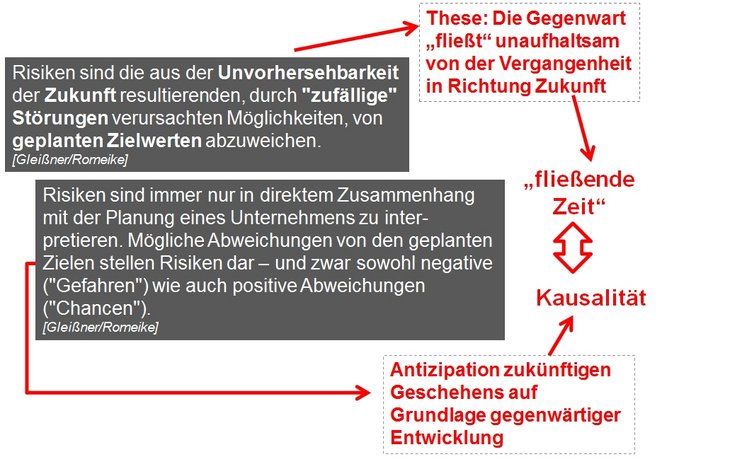
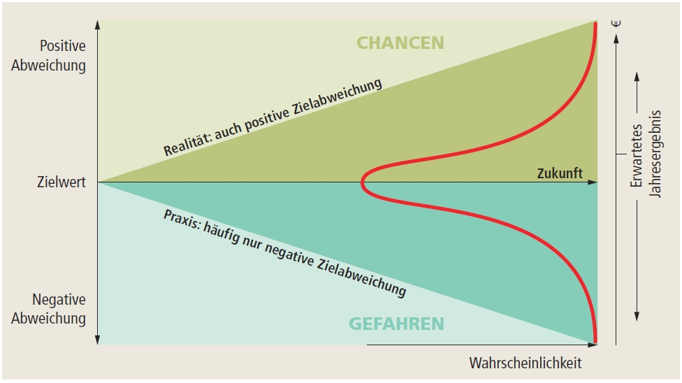
Entrepreneurial activity is always associated with risk. The job of risk management is to systematically identify opportunities and risks and to evaluate them in terms of their potential impacts on the company. The concept of risk can thus be defined as a spread around an expected value. According to this definition, both positive variations (opportunities) and negative variations (hazards) can exist.
Objectives of risk management
One of the tasks of risk management in companies is to reduce the spread or fluctuation of profit and cash flow, and to increase the overall planning security. This can lead to the following positive effects for the company [see Gleißner/Romeike 2005, p. 28 onwards, and Romeike, Hager 2009, p. 108]:
- Reducing fluctuations increases predictability and controllability in the company, which has a positive impact on the expected level of returns.
- A predictable development in cash flows reduces the probability of having to unexpectedly resort to expensive external sources of finance.
- Reducing the risk-related fluctuation in future cash flows cuts the capital costs and has a positive impact on the company's value.
- Stable profit performance with a high probability of adequate debt servicing capability benefits capital markets, which is reflected in a good rating, a relatively good financial framework and favourable credit conditions.
- Stable profit performance and high risk bearing ability (capital resources) reduces the probability of insolvency.
- Stable profit performance and a lower probability of insolvency benefit employees, customers and suppliers, which makes it easier to recruit qualified staff and establish long-term relationships with customers and suppliers.
- With a progressive tax scale companies with fluctuating profits are also at a disadvantage compared to companies with consistent profit performance.
Risk management as a control loop
An efficient risk management process functions in a similar way to the human organism or other network structures in nature. In a human organism, the brain, heart and nervous system work together. Networks are adaptable and flexible, have common objectives, interact and avoid hierarchies. Network structures are scalable and exceptionally resilient.
Applied to the risk management process, this means that different sensors and senses (such as the eyes, ears, nerves or early warning indicators) detect risks and communicate them to a central point (brain or risk manager). The overall strategic direction of the system (company) determines the understanding of risk. In this context it is important not to view the strategic dimension of risk management separately from strategic business management (business strategy).
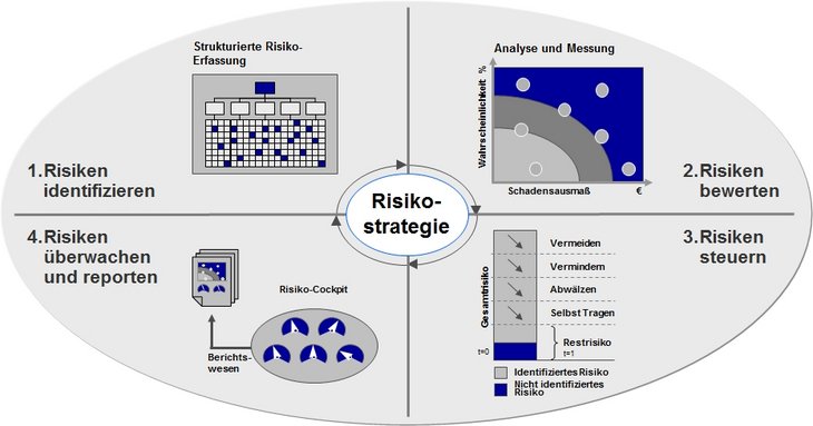
Strategic risk management represents the integrative framework and the foundation of the entire risk management process. It primarily involves formulation of risk management objectives in the form of a "risk strategy". Before risk management can be implemented and conducted as a continuous process, the basic principles in terms of the general conditions (for example risk appetite, risk bearing ability), organisation (functions, responsibilities and information flow) and the actual phases of the process must first be defined.
Operational risk management (see figure above) includes the process of systematic and ongoing risk analysis for the business processes. The aim of risk identification is early detection of "developments that cold jeopardise the continued existence of the company", i.e. the fullest possible detection of all potential risk causes, losses and potential disruptions. The key to an efficient risk management process is that it is integrated into the company's processes as a continuous process, in the sense of a control loop.
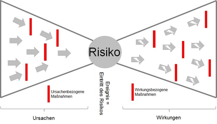
Procurement of information is the most difficult phase of the entire process and is a key function in risk management as this step provides the information basis for all subsequent phases. Ultimately, only risks that have actually been detected can be evaluated and controlled. In the risk identification phase, it is important to differentiate between causes, the potential variations from plans/targets (risks) and the effects.
Differentiating between risk causes or drivers and effects can be clearly illustrated in a bow tie diagram. The measures relating to the causes and effects can also be shown.
Early warning systems for risk identification
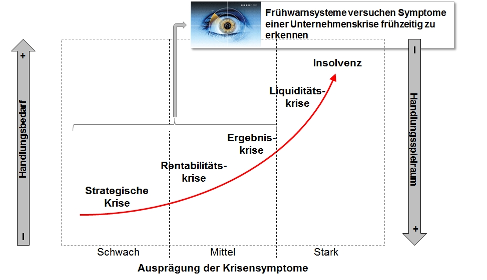
One of the most important instruments in risk identification are early warning systems, which contain early warning indicators (such as economic or purchasing indices or internal factors such as employee dissatisfaction or process quality) to draw their users' attention to latent (i.e. existing but hidden) risks in good time, leaving sufficient time to take appropriate measures to avert the occurrence of the risk or reduce its impact (see Romeike 2008, p. 65, and Romeike 2005, p. 22-27]. Early warning systems thus give a company time for responses and optimise controllability.
Identification of risks
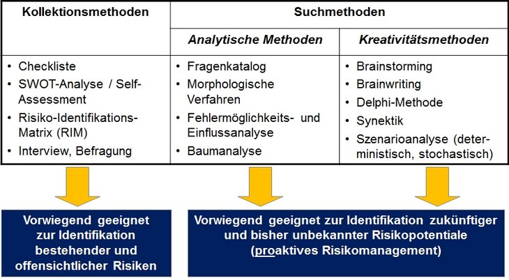
The choice of risk identification measures depends significantly on the specific risk profiles of the company and the industry. In practice, the individual methods and tools need to be combined. The figure below provides an overview of the different methods used in practice. When recording risks, checklists, workshops, inspections, interviews, organisational plans, balance sheets and damage statistics are useful. The results of the risk analysis are used to produce a risk inventory.
The risks identified then have to be analysed and evaluated in detail in the subsequent step of the process. The aim of this should be to obtain a meaningful risk measure, where possible applicable to all risk categories.
In practice, risks are traditionally quantified in terms of the extent of the losses and the probability of occurrence (mathematically, this is based on a binomial distribution). The expected value (for discrete random variables) is determined in two dimensions by multiplying the probability of occurrence by the extent of loss (risk dimension, risk potential, scope). The expected value E(X) or μ for a random variable (X) is the value that is (normally) calculated as the mean of the results from repeated repetitions of the underlying experiment. It determines the localisation (position) in a distribution and is comparable with the empirical arithmetic mean in a frequency distribution in descriptive statistics. In many cases the law of large numbers ensures that the sample mean converges with the expected value as the sample size increases.
In this brief introductory text, we cannot go into the different evaluation methods used in practice in more detail [for a more in-depth explanation, see Romeike/Hager 2013].
The risk manager's tool kit provides a great variety of methods and analysis options. The choice of tools and methods is primarily determined by the available data for individual risks. For quantifiable risks, the potential loss can be split into three areas: Expected losses, statistical losses and stress losses.
The "expected loss" (also referred to in financial services as standard risk cost) reflects the average inherent losses associated with a business activity. These are included in planning and – where permitted by the applicable accounting standards – are deducted directly from revenue.
The statistical loss (or "unexpected loss") is the estimated variation in the effective loss from the expected loss over a particular time horizon and assuming a specified confidence interval (also known as the confidence range).
The stress loss is the loss that can be triggered by extreme events (high severity / low frequency risks). In practice, as sufficient historic risk or loss data is not generally available for these kinds of extreme events, we either have to use theoretical random distributions or use stress tests to analyse potential stress scenarios. For potentially catastrophic events that occur very rarely but produce fatal amounts of loss, in practice we also use "extreme value theory" (EVT) or the peaks over threshold (PoT) method [see Embrechts/Klüppelberg 1997].
Evaluation of risks
In practice, many companies only use a simple system that classifies the probability of occurrence and the extent of loss using just a few levels – normally based on an expert assessment.
| Probability of occurrence | |
|---|---|
| 1 = High probability of occurrence (frequent) | Occurrence within a year is expected; or occurrence empirically in the past 3 years |
| 2 = Medium probability of occurrence (possible) | Occurrence within 3 years is expected; or occurrence empirically in the past 8 years |
| 3 = Low probability of occurrence (rare) | Occurrence within 8 years is expected; or occurrence empirically in the past 15 years |
| 4 = Unlikely | Risk has not yet occurred, even in comparable companies. However, the risk cannot be ruled out altogether. |
| Extent of loss | |
|---|---|
| 1 = Catastrophic risk | Occurrence of the risk would jeopardise the company's existence |
| 2 = Major risk | Occurrence of the risk would force a short-term change in the company's objectives or strategy |
| 3 = Medium risk | Occurrence of the risk would force a medium-term change in the company's objectives or strategy |
| 4 = Minor risk | Occurrence of the risk would force the company to change its methods and processes |
| 5 = Trivial risk | Occurrence of the risk has no impact on the value of the company |
In practice, the initial relevance assessment is carried out by competent experts who base their conclusions on the realistic maximum loss.
For example, they divide risks into five relevance classes from "insignificant risk" to "risk jeopardising existence". The table below shows examples of different relevance classes.
Relevance is viewed as the overall significance of the risk for the company. This is a further risk measure and depends on the following factors:
- Medium burden on profit (expected value),
- Realistic maximum loss,
- Duration of effect.
A further advantage of the relevance assessment is that it provides a simple description of the severity of a risk, thus making communication of relevant risk information easier.
Either a "top down" or a "bottom up" evaluation methodology can be adopted. If the evaluation is based on a top down method, the company's focus is on the known consequences or effects of the risks (see bow tie diagram). Data from the profit and loss account, such as revenue, costs or operating profit is analysed in terms of its volatility. A top down approach has the advantage of providing a relatively quick outline of the major risks from a strategic perspective. However, this "macro perspective" can lead to certain risks being missed or correlations between individual risks not being correctly evaluated.
| Relevance class | Effect on risk bearing ability | Explanations |
|---|---|---|
| 1 | Insignificant risk | Insignificant risks that do not noticeably influence annual net profit or the value of the company. |
| 2 | Medium risk | Medium risks that have a noticeably detrimental effect on annual net profit. |
| 3 | Significant risk | Significant risks that have a major influence on annual net profit or lead to a noticeable reduction in the company's value. |
| 4 | Severe risk | Severe risks that lead to an annual net loss and significantly reduce the company's value. |
| 5 | Risk jeopardising existence | Risks jeopardising existence that are very likely to jeopardise the continued existence of the company. |
When using bottom up methods, the causes (see bow tie diagram) of the different risks are the focus of the analysis. An attempt is made to deduce and evaluate the possible consequences of a risk occurring for the company. This requires a thorough analysis of processes and the associated cause/effect chains and dependencies. The advantage of bottom up methods is that they enable all areas of the business and all processes to be included and analysed. However, the bottom up approach involves many times the amount of work. In practice, a combination of top down and bottom up methods is generally used.
The risk manager's tool kit provides a great variety of methods and analysis options. The choice of tools and methods is primarily determined by the available data for individual risks. For quantifiable risks, the potential loss can be split into three areas: Expected losses, statistical losses and stress losses.
We are unable to deal with the individual risk evaluation methods in detail here (for a detailed introduction and in-depth explanation of the various methods, refer to the publication by Romeike/Hager 2013). In addition, the RiskNET Glossary provides a brief introduction to the key methods. Supplementary information can also be found in the Risk management methods section.
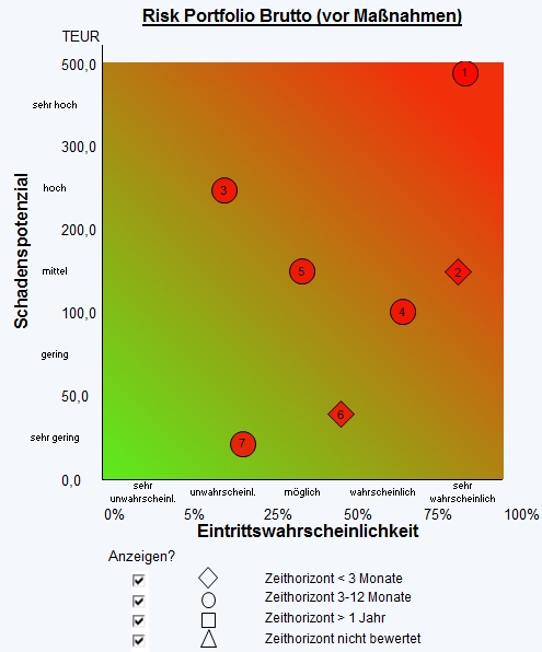
The results of the risk evaluation can be transferred to the risk inventory (or risk catalogue). If the probability of occurrence and the resulting effect (expected values for impact, extent of loss etc.) have been quantified based on the bottom up or top down methods outlined above, they can be represented in a risk map (also known as a risk matrix or heat map). The figure below shows an example of a risk map. A risk map provides a (greatly simplified) overview of a company's risk portfolio and gives decision makers an initial basis for risk control and monitoring.
Formally, the risks shown in a risk map are binomially distributed risks. They have just two states: Either the risk occurs (and loss occurs according to the defined level of loss) or it does not occur.
Here is a specific example based on the risk map shown: If Risk 6 occurs (the probability is 50 percent that the risk will occur and 50 percent that it will not; the equivalent of tossing a coin), the level of loss is exactly 50,000 EUR. However, in practice it tends to be the case that both the probability of the risk occurring and the level of loss will be unknown.
The majority of risks cannot be described using the underlying Bernoulli process, for example because the number of "tries" n (or potential risk occurrences) is not known or the probability of success p is also unknown. We only need to think of the uncertainty surrounding demand or the development of exchange rates and raw material prices – here the probability of a potential variation from plan occurring is 100 percent. Only the potential fluctuation range or volatility is unknown.
Scenario-based approaches, creativity methods and simulation methods help to identify and evaluate events threatening the company's existence (for example using an appropriate distribution function, such as a triangular distribution, a PERT distribution, a normal distribution or a Poisson distribution).
The academic Benoît B. Mandelbrot, best known for his pioneering work in fractal geometry and chaos research, summed things up perfectly long before the most recent market turbulence: "If someone is building a ship, he's not interested in when exactly the next storm will come. He builds the ship to survive any conceivable storm."
Aggregation of risks
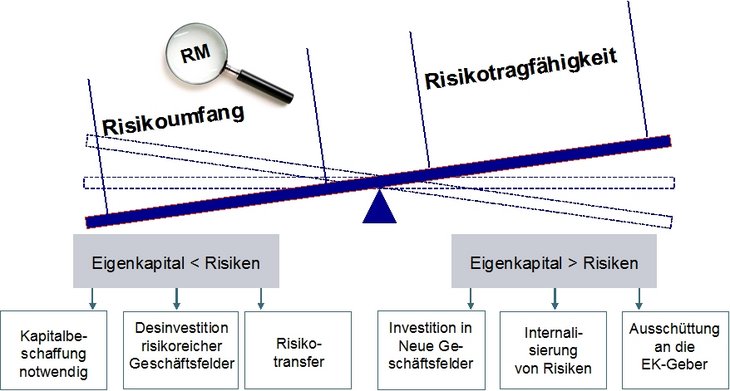
Aggregation of the identified relevant risks is necessary because in reality they have a combined effect on profit and capital. Thus, it is obvious that all risks are a joint burden on a company's risk bearing ability (see risk bearing ability figure below).
In simple terms, risk bearing ability is determined by two factors, namely capital resources and liquidity reserves. Assessing the overall extent of risk allows us to draw conclusions about whether a company has sufficient risk bearing ability to actually withstand the risks that the company is exposed to and thus to guarantee the company's continued existence.
The need for this kind of method is emphasised by auditors, as shown by the following statement from the IDW (German Institute of Auditors) on the Corporate Sector Supervision and Transparency Act (IDW PS 340):
"Risk analysis includes an assessment of the reach of the identified risks in terms of probability of occurrence and quantitative effects. This includes analysis of whether individual risks, which are of secondary importance when viewed individually, can interact or aggregate cumulatively into a risk that jeopardises existence over time."
Aggregating risks to give a total risk position can essentially be done in two ways, analytically or by simulation. The analytical method requires an assumed distribution. The variance/covariance method is an analytical process to determine the value at risk, a total risk position given by adding together various individual risks. The term is frequency used synonymously with the more correct description "delta normal method" and corresponds to the original VaR model from J.P. Morgan. The stochastics of the risk factors (volatilities and correlations) are described using a covariance matrix, i.e. multivariate normally distributed changes in the risk factors are assumed. The volatilities (standard deviation) of the risk factors are used to calculate the value at risk for the individual risk factors, and the correlation matrix is then used to aggregate them to the relevant risk consolidation level to give the overall risk position.
For methodologically clearer risk aggregation, we should choose methods that
- are able to capture risks described by any probability distributions,
- take into account non-additive (for example multiplicative) links between risks, and
- create a context for corporate planning, as risk management ultimately aims to highlight a company's planning reliability and capital requirements consistently with its actual planning.
Against this measure, "historic simulation", which is frequently used in risk management particularly by banks, often disqualifies itself, at least partly.
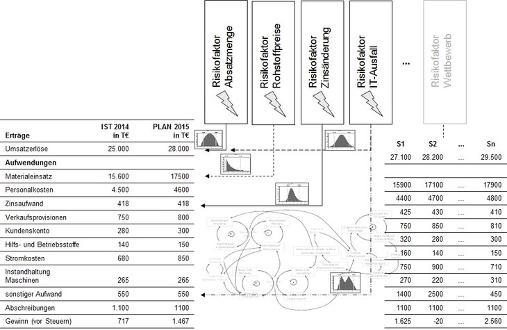
Therefore simulation-based methods for aggregation of risks are adopted (for example based on the Monte Carlo simulation). This initially involves assigning the effects of individual risks to specific items in the planned profit and loss account or the planned balance sheet: For example, an unscheduled increase in the cancellation rate will have an impact on various items in the profit and loss account.
Assignment of risks to business planning items is a requirement for using risk aggregation to determine the "total risk exposure". Risks can be modelled as a fluctuation range around a planned value (for example +/- 10 % fluctuations for defined market risks). The following figure shows the fundamental principle of aggregating risks and the sensitivity analysis. S1 to Sn show the different future paths of the output variables – based on the modelled risks (= input factors).
Looking at the different scenarios in the simulation runs (see figure below) illustrates that each simulation run produces different combinations of risk and output factor developments. Each step provides a simulated value for the target variable (for example EBIT or cash flow). The total of all simulation runs provides a "representative sample" of all possible risk scenarios for the company and allows an insight into potential future scenarios. The calculated values of the target variable result in aggregated probability distributions (density functions), which can then be used for further analyses. Another result is that stress paths can be analysed and sensitivity analysis can be used to calculate the severity of the effect of individual risks on the output variables.
Only the total risk exposure – resulting from the risk aggregation – allows a sound initial assessment of the company's risk bearing ability, which largely determines the risk financing or risk transfer measures adopted. In this context, calculation of the imputed capital resources costs – a key component of the total risk costs – is very important. Risk transfer solutions (for example insurance policies) ultimately substitute scarce and relatively expensive capital resources.
The imputed capital resources costs are given by multiplying the capital requirement by the capital resources cost rate, which depends on the accepted probability of default and the expected return on alternative investments (for example on the share market).
Risk control
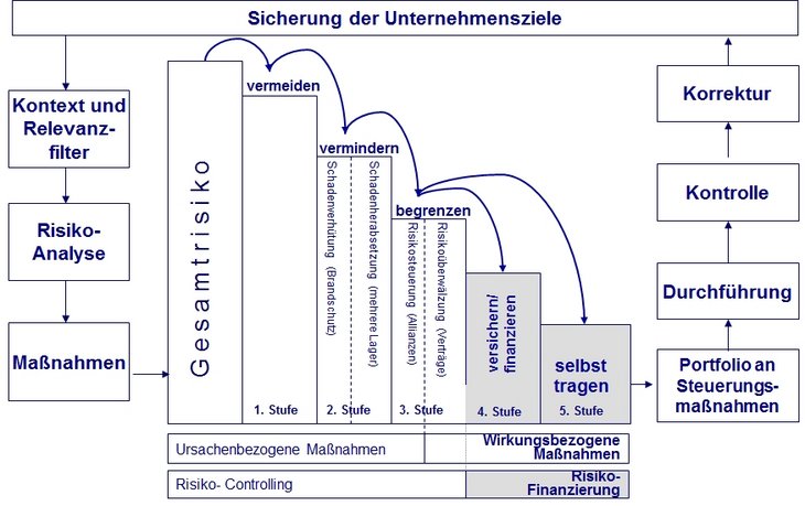
Risk control and monitoring plays a key role in the overall risk management process (see figure). The aim of this phase is to positively change the company's risk position and to achieve a balanced ratio between revenue (opportunity) and potential loss (risk), in order to increase the company's value. Risk control and monitoring encompasses all mechanisms and measures designed to influence the risk situation, by reducing the probability of occurrence and/or the extent of loss. Risk control and monitoring should be consistent with the objectives defined in the risk strategy and the general corporate objectives. The aims of this phase in the process are to avoid unacceptable risks and to reduce and transfer unavoidable risks to an acceptable level. Optimum risk control and handling is the approach that increases the company's value by optimising its risk position.
In terms of control and management of risks, there are essentially three alternative strategies. A preventive (or aetiological) risk policy aims to actively avoid or prevent risks by eliminating or reducing the corresponding causes (see bow tie diagram). An attempt is made to improve the risk structure by reducing the probability of occurrence and/or the consequences of individual risks.
In contrast to these active control measures that directly address the structural causes of risk (probability of occurrence, extent of loss), a corrective (or palliative) risk policy consciously accepts the occurrence of a risk. The aim of a passive risk policy is not to reduce the probability of occurrence or the consequences of the risks, i.e. the risk structures are not changed. Instead, the risk taker attempts to implement appropriate measures for risk mitigation. The aim of this risk mitigation is to prevent or reduce the effects of the risk occurring (see bow tie diagram). For example, this can involve the frequently practised shifting of risks to other risk takers (such as insurance companies or the capital market). If a risk occurs, as well as providing the required liquidity, this cushions the negative consequences on profitability.
Further literature:
- Embrechts, P./Klüppelberg, C./Mikosch, T. (1997): Modelling extremal events for insurance and finance, Berlin 1997.
- Gleißner, W./Romeike, F. (2005): Risikomanagement – Umsetzung, Werkzeuge, Risikobewertung [Risk Management - Implementation, Tools, Risk Evaluation], Freiburg i. Br. 2005.
- Romeike, F./Hager, P. (2009): Erfolgsfaktor Risk Management 2.0 – Methoden, Beispiele, Checklisten: Praxishandbuch für Industrie und Handel [Success Factor Risk Management 2.0 - Methods, Examples, Checklists: Practical Handbook for Industry and Commerce], 2nd edition, Wiesbaden 2009.
- Romeike, F./Hager, P. (2013): Erfolgsfaktor Risk Management 3.0 – Methoden, Beispiele, Checklisten: Praxishandbuch für Industrie und Handel [Success Factor Risk Management 2.0 - Methods, Examples, Checklists: Practical Handbook for Industry and Commerce], 3rd edition, Wiesbaden 2013.
- Romeike, F. (2008): Gesunder Menschenverstand als Frühwarnsystem (Gastkommentar) [Healthy Judgement as an Early Warning System (Guest Commentary)], in: Der Aufsichtsrat, Issue 05/2008, page 65.
- Romeike, F. (2005): Frühwarnsysteme im Unternehmen, Nicht der Blick in den Rückspiegel ist entscheidend [Early Warning Systems in Business, Looking in the Rear View Mirror is Not The Critical Factor], in: RATING aktuell, April/Mai 2005, Heft 2, S. 22-27.
![The risk management process [Image source: © Adobe Stock] The risk management process [Image source: © Adobe Stock]](/fileadmin/user_upload/Headerbilder/Headerbild_Risk_Management_Prozess.jpg)
